Blog
Search our Blog for latest news, use cases, blog entries, etc.
Top keywords: Wi-Fi, Low Latency, HFC
Blog
Become a Wi-Fi expert
Read More
Is L4S the real latency killer?
Read More
Unleashing the Power of L4S in Access Networks
Read More
White Paper Alert: Unveiling the Power of L4S and Wi-Fi 7
Read More
The 10G revolution: DOCSIS 4.0 offers over 10 times the current speed
Read More
Webinar: Is Latency the holy grail to fantastic user experience?
Read More
Prove you have the best Wi-Fi at Excentis
Read More
Excentis supports first live DOCSIS 4.0 test by Liberty Global & VodafoneZiggo
Read More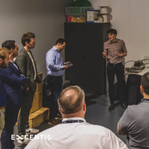
Low Latency DOCSIS training for Virgin Media O2
Read More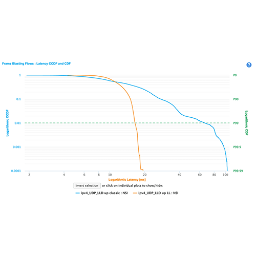
Bouygues Wi-Fi 6E gateway and CPE device testing with ByteBlower
Read More
Lowering latency in the PŸUR DOCSIS network
Read More
LTE Interference Testing
Read More
Let's advance
networks together
We would welcome the opportunity to work with you to optimize, innovate and assure the robustness of your networks. And we put our heart into it, our work is our passion.

Jan De Beule
EMEA

Charlie Viaene
AMER-APAC
Any questions?
We're humbled to be trusted by the best


