Measuring throughput: effect of used TCP settings
Measuring throughput using TCP seems an easy task: just send data over a TCP session and the protocol will automatically seek the maximum network capacity for you. If you’re in luck this will give you satisfying results, but what if it doesn’t? Exactly which parameters should you play with to optimize your performance? Let’s find out!
Size matters
First we focus on the flow control mechanism of TCP. The receiving side of a TCP session is in charge of this. By reporting its current receive window size it lets the sender know how many bytes it is willing to accept. This way the receiver will never get overwhelmed with data.
When it comes to performance, choosing an optimal size for this receive window is important. Pick it too small and it will limit the sender more than necessary. Pick it too large and it can lead to inefficient retransmissions of packets in case of packet loss.
So how do we find the optimal receive window size?
In essence, a receive window controls the amount of unacked data which can exist between the sender and receiver. We can easily calculate this by multiplying the network bandwidth with its round-trip time. The result of this calculation is called the Bandwidth-delay product (BDP).

Let’s try this out for a network with an expected throughput of 200 Mbps, an RTT of 30 ms and a MTU of 1500. In this case the BDP will be:

This tells us that we should be able to receive 750,000 Byte if we want to use our network capacity to the limit. However this value is not directly usable as receive window size, because it exceeds the maximum possible TCP window size of 65,535 Bytes.
To solve this we need to use the TCP window scale option defined in RFC 1323 . The value of this option specifies how many times the receive window size needs to be left-shifted to obtain the “to be used” window size. A left shift is equivalent to multiplying the window size with the factor 2N (where N is the window scale).
After some mathematical magic we can derive a formula for the window scale (N):

For “initial window size” we will choose a multiple of the Maximum Segment Size (MSS).

Let’s test it out on our example:
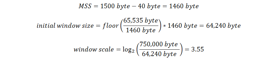
Because half a scale is not usable we round it up to 4.
That’s it! For our example the recommended window size is 64,240 byte with a window scale of 4.
Another possibility would be to select a smaller window size and a bigger window scale factor. One of the benefits of this is that during transmission the window size can then be dynamically adjusted. To do this, TCP messages contain timestamps which make it possible to calculate the RTT during the TCP session.
The window scale, on the other hand, is fixed during the entire connection, so it is important to choose a suitable value right from the start.
Getting SACKed boosts performance
Besides the receiver, the network you are sending through has bottlenecks as well. This is where the TCP congestion avoidance mechanism comes into play.
Tahoe, Reno, New Reno, Vegas, Hybla, BIC, CUBIC, Compound… These are just a few of the existing implementations you can pick from, but the one you should be looking at is called Selective ACK (SACK).
Other popular mechanisms like Tahoe, Reno and New Reno have certain shortcomings which impact performance. The main problem is that received out-of-order segments don’t get ACKed which can lead to unnecessary retransmission of correctly received data in case of packet loss. These implementations also encounter problems when multiple segments get lost in the same window.
A quick overview:
| Tahoe | Reno | New Reno | |
|---|---|---|---|
| How it works | Enter fast retransmit state after 3 duplicate ACKs When done, fall back to slow start (congestion window size is reset to 1) | After fast retransmit, enter fast recovery: the congestion window size is not reset, but halved and incremented with 3 After “normal” ACK: exit fast recovery | Sender remembers number of last segment sent before entering fast recovery Stays in fast recovery stage until ACK is sent which covers last remembered segment => all segments lost before entering fast recovery will be resent |
| Problems | Duplicate ACKs tells sender receiver is still reachable => Large, avoidable performance drop | Does not handle multiple lost segments in one window very well | For every resubmitted packet, newReno has to wait for a new ACK before it can decide which other packets needs to be resubmitted. => It takes one RTT to detect each packet loss |
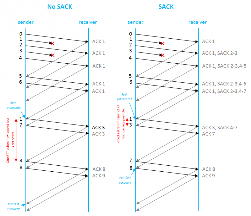
SACK deals with these issues by using Selective ACKs.
When an out-of-sequence packet reaches the receiver, selective ACKs are sent which contain additional blocks telling the sender which segments are received correctly. This way the sender gets a complete picture of which packets needs to be retransmitted and which packets don’t. Simply put, SACK adds extra information to ACK messages to make it possible to also ACK out-of-sequence segments.
SACK does not change the underlying TCP congestion control algorithms. Which means it still uses the well known Slow Start and Fast Retransmission + Recovery mechanisms as used by TCP Reno.
Conclusion
Measuring TCP throughput is indeed not as straightforward as it first seems. When results are not as expected investigating the used TCP stream settings is one of the first things to check when looking for possible bottlenecks. Optimizing the receive window size, enabling window scale option and using SACK can greatly improve your performance.