Low Latency Series Part 2: What is Low Latency DOCSIS and why?
Internet has grown tremendous the last 20 years. It provides possibilities we couldn’t even think of 20 years ago. The more possibilities the internet provided; the more bandwidth was needed. Evolution from dialup internet to DSL and cable internet and fibre made this all possible.
But an increase in bandwidth is not always the solution. Certain services can’t be improved by just adding additional bandwidth. These services need real-time behaviour. Think at applications such as web meetings and live video, but also online gaming or medical applications. For these applications, latency and jitter are at least equally important as throughput.
End-to-end latency is complex, but with Low-latency DOCSIS, the cable access network is not going to be the weakest link in the latency chain. DOCSIS networks typically have a round trip time of 10ms when idle. Under heavy load, this can increase with spikes to 1 second. Latency sensitive application will perform badly in such situations while the bandwidth is not the issue. Low Latency DOCSIS is added to the DOCSIS 3.1 specification to handle this problem. It will keep the round trip time around 1 millisecond (for specific services), even under heavy load.
Latency, it’s not only the network!
When talking about latency, we mostly think of latency introduced by the network. Probably because this is covering the longest distance. It is important to note than many other components introduce latency. If we look at gaming, the game console itself will introduce latency. And when the image is created, it takes between 16 to 33ms to reach the screen over a typical HDMI connection.
- Playstation 4 ~50ms
- Xbox One: ~60ms
- Wi-Fi latency: 2-4 ms
But even our brains introduce latency:
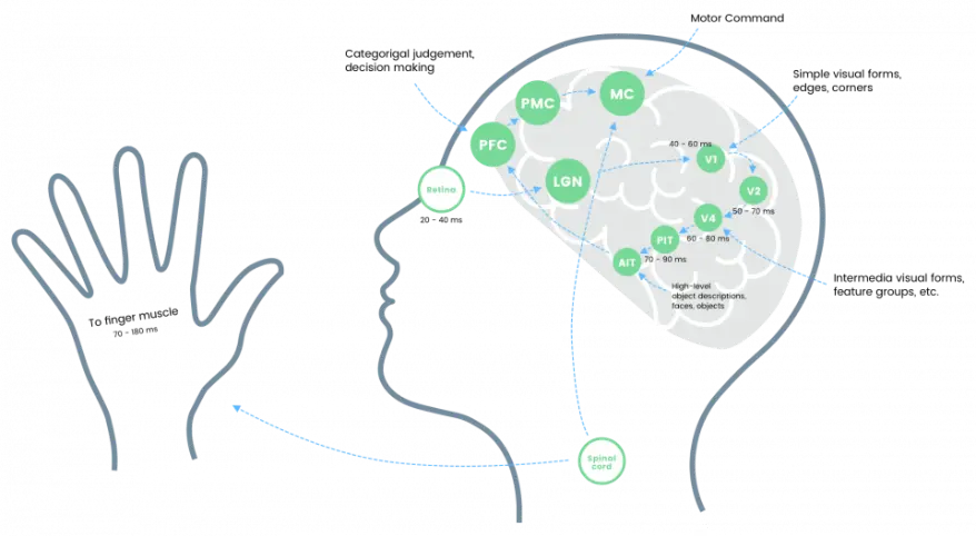
As we are currently unable to replace the brain, we will focus on the access network in this blog post.
Latency we can’t reduce
Latency in a network is caused by:
- Propagation delay, mainly influenced by the distance between sender and receiver
- Serialisation and deserialization
- Buffering and queuing in the network
The latency introduced by the geographical distance between the sender and receiver can not be ignored.
Here are some optimistic examples when using fibre optics:
| Route | Distance (km) | Fibre (one direction, ms) | Fibre (round trip, ms) |
|---|---|---|---|
| New York – San Francisco | 4148 | 21 | 42 |
| New York – London | 5585 | 28 | 56 |
| New York – Sidney | 15993 | 80 | 160 |
How LLD reduces latency
To minimize the impact of the network on latency, LLD focusses on the biggest sources for latency: Media acquisition and Queuing.
Media acquisition delay is introduced by the scheduling mechanism needed on a shared medium such as coax. This mechanism will ensure only one user is using a transmission slot at the same time. This will typically introduce an additional round trip time of 2 to 8 ms. To reduce this latency, LLD uses DOCSIS MAP intervals. Besides that, it uses PGS (Pro-active Grant Service). This allows a modem to send upstream traffic without requesting it.
The biggest source of latency is queuing delay. As most applications rely on TCP (or Quic) and similar protocols to have as much bandwidth as possible, the ‘congestion avoidance’ algorithms will adjust to the link which is the speed. In most situations, this is the access network. Buffers and queues on that link will be stressed to the limit. It will optimise bandwidth but increase the latency on this link.
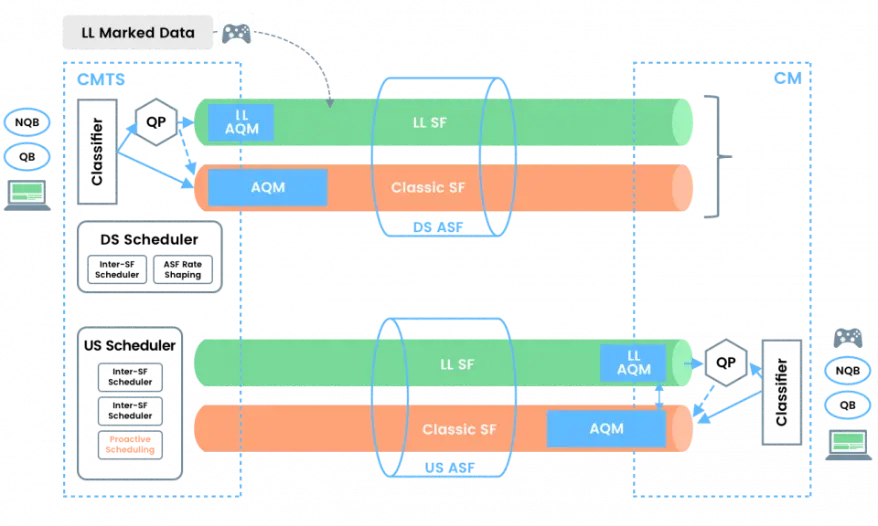
Low Latency DOCSIS resolves the Queueing latency by using a dual queuing approach. Applications which are not queue building (such as online gaming applications) will use a different queue than the traditional queue building applications (such as file downloads). Non-queue building traffic will use small buffers – minimizing the latency – , queue building traffic will use larger buffers – maximizing the throughput.
LLD allows operators to group up- and downstream service flows to enable low-latency services. Certain service flows will carry the non-queue building application traffic, while the other will carry the queue-building traffic. On the other hand, the operator can configure the service rate shaping on the Aggregate Service Flow, which combines the NQB and QB service flows in one direction.
In our next article, we will demonstrate how NQB and QB traffic can be detected and will perform our first tests with ByteBlower!